
Chapter 7 Exercise: Numerical Modeling of Balanced and Unbalanced Transmission Lines
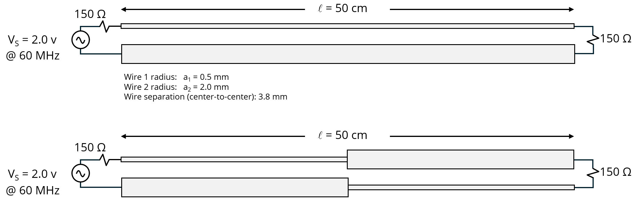
Experimentation with numerical modeling tools is a great way to learn about the behavior of circuit parasitics and electromagnetic wave propagation. This lab demonstrates how changes in electrical balance cause mode conversion in transmission lines.
Preparation: Students need to know how to use a 3D EM modeling code.
Equipment Required:
- 3D EMC modeling code capable of modeling open systems of conductors
Procedure:
Step 1: The first configuration to model is illustrated in the top half of the figure. It is a transmission line consisting of two parallel wires. Both wires are 50 cm long. One wire has a radius equal to 0.5 mm, and the other wire has a radius of 2.0 mm. The center-to-center wire separation is 3.8 mm. One end of the transmission line is driven by a 2.0-volt, 150-Ω source at a frequency of 60 MHz. The other end of the transmission line is terminated with a 150-Ω resistance.
Step 2: Calculate the current on Wire 1 and the current on Wire 2 at a location 12 cm from the source. The two values should have nearly the same amplitude with opposite polarities. Use these values to calculate the differential-mode and common-mode current 12 cm from the source. (Theoretically, there is no common-mode current on this transmission line. However, numerical noise due to finite precision calculations and the grid used to create the model ensure that the calculated result will never be exactly zero.)
Step 3: Use the model to determine the radiated electric field strength at a distance of 3 meters from the center of the transmission line in a direction perpendicular to the length of the transmission line. Compare this to the calculated value of the radiated electric field from a wire pair due to differential-mode current (Equation 3.62 in the book).
Step 4: Use the same modeling code to model the second configuration shown in the figure. In the center of the transmission line, the thin wire becomes thick, and the thick wire becomes thin. The cross-sectional geometry of the right and left halves of the transmission line is the same, only rotated 180 degrees. The characteristic impedance of both halves is the same.
Step 5: Calculate the current on Wire 1 and the current on Wire 2 at a distance of 12 cm from the source. Use these values to calculate the differential-mode and common-mode current 12 cm from the source.
Step 6: Use the model to determine the radiated electric field strength at a distance of 3 meters from the center of the transmission line in a direction perpendicular to the length of the transmission line. Compare this to the calculated value of the radiated electric field from a wire pair due to differential-mode current (Equation 3.62 in the book) and common-mode current (Equation 3.61 in the book). Note that the common-mode current has a triangular wave shape, so the value 12 cm from the source is approximately the average value along the entire length of the line.
Step 7: How well do the equations for the radiated emissions from common-mode and differential-mode currents on a wire segment in the book (Equations 3.61 and 3.62) agree with the emissions from the common-mode and differential-mode currents in the model? Explain any significant differences.
Notes:
If the students have access to a 2D static modeling code, they can calculate the imbalance factor of the transmission line. The common-mode source created by the change in imbalance in the second configuration has an amplitude equal to VDM times Δh. Students can turn off the differential source and drive the two halves of the second configuration with the equivalent common-mode source. This will yield approximately the same radiated field as the original configuration.