Inductance

Capacitance was defined in terms of electric charge generating an electric field resulting in a voltage proportional to the charge. Inductance is a property associated with electric current that produces a magnetic field resulting in a coupled magnetic flux proportional to the current. In the same way that capacitance helps engineers quantify electric-field coupling, inductance helps quantify magnetic-field coupling.

A conductor of any shape can hold an electric charge, so conductors of any shape can have a self-capacitance. However, current flows in loops, so self-inductance is a property of current loops. And just as the electrical field that couples two conductors can be quantified as a mutual capacitance, the magnetic field that couples two current loops can be quantified in terms of a mutual inductance.

In the EMC literature, it’s not uncommon to see references to the inductance of a wire, trace, via, or ground strap. These things contribute to the inductance of a current loop. However, their contribution can only be determined when the rest of the loop is identified. Concepts such as partial inductance and branch inductance have been developed to model geometries in which the loop is not apparent, or multiple loops exist. These concepts can be helpful, but any application of inductance will depend on how the current loop is closed. In this section, we’ll review several inductance concepts, starting with the most basic.

External Inductance of a Wire Loop

Just as capacitance is a measure of the total electric flux that couples two conductive objects relative to their static potential, inductance is a measure of the total magnetic flux coupling two current paths relative to their steady-state current. A single wire loop has a self-inductance just as a single conductive object has a self-capacitance. Two wire loops can have a mutual inductance just as two conductive objects can have a mutual capacitance.

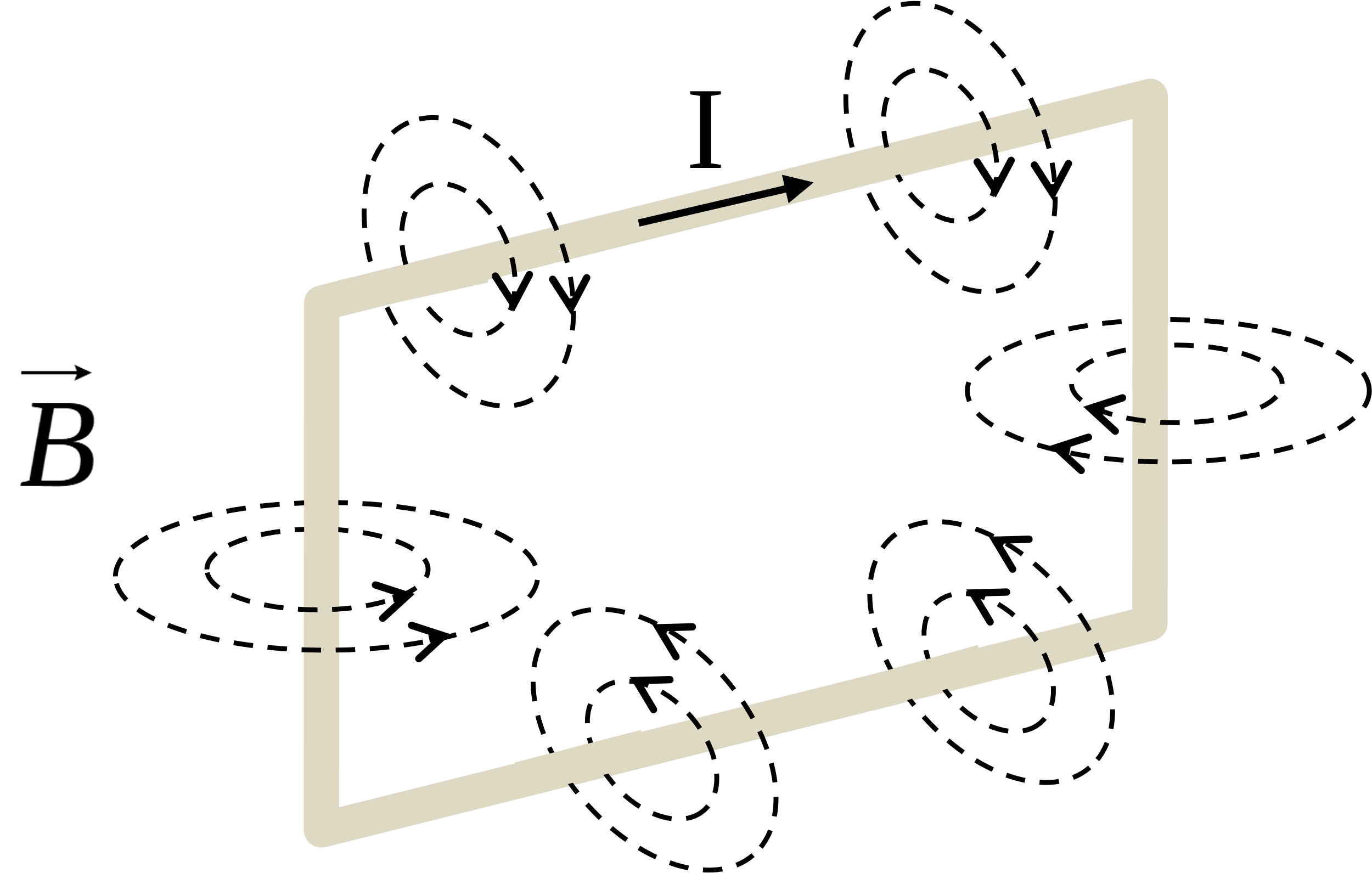
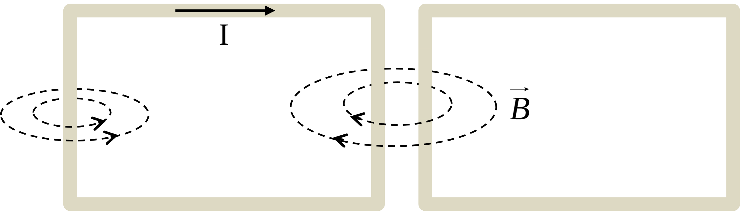
Figure 1. Magnetic flux coupling a current loop.

Figure 1 illustrates lines of magnetic flux wrapping the wires in a current loop. Lines of magnetic flux form continuous loops that encircle the source current. The direction of the flux lines can be determined by pointing the thumb of the right hand in the direction of the current. The fingers of the right hand will then curl in the direction of the magnetic flux created by the current. Integrating over all the flux lines passing through the loop, we could calculate the total magnetic flux coupling the loop as,

(1)

Ψ= S B ds webers MathType@MTEF@5@5@+= feaahWart1ev3aaatCvAUfeBSjuyZL2yd9gzLbvyNv2CaerbpbxzUb YuH52CaeXatLxBI9gBaebbnrfifHhDYfgaruatPjwzYfgDP9MBGmvz YLMzaibaiKc9yrVq0xXdbba91rFfpec8Eeeu0xXdbba9frFj0=OqFf ea0dXdd9vqaq=JfrVkFHe9pgea0dXdar=Jb9hs0dXdbPYxe9vr0=vr 0=vqpWqaaeaabaGaaiaacaqabeaadaabamaaaOqaaiabfI6azjabg2 da9maapefabaWaa8HaaeaacaWGcbaacaGLxdcacqGHflY1daWhcaqa aiaadsgacaWGZbaacaGLxdcacaaMi8oaleaacaWGtbaabeqdcqGHRi I8aOGaaGzbVlaabEhacaqGLbGaaeOyaiaabwgacaqGYbGaae4Caaaa @4EBD@  

where the unit of magnetic flux is the weber (Wb), and B MathType@MTEF@5@5@+= feaahWart1ev3aaatCvAUfeBSjuyZL2yd9gzLbvyNv2CaerbpbxzUb YuH52CaeXatLxBI9gBaebbnrfifHhDYfgaruatPjwzYfgDP9MBGmvz YLMzaibaiKc9yrVq0xXdbba91rFfpec8Eeeu0xXdbba9frFj0=OqFf ea0dXdd9vqaq=JfrVkFHe9pgea0dXdar=Jb9hs0dXdbPYxe9vr0=vr 0=vqpWqaaeaabaGaaiaacaqabeaadaabamaaaOqaamaaFiaabaGaam OqaaGaay51Gaaaaa@3A64@  is the flux density in Wb/m2. The unit of inductance is the henry (H), and the self-inductance of the loop is,

(2)

L= Ψ I henries. MathType@MTEF@5@5@+= feaahWart1ev3aqatCvAUfeBSjuyZL2yd9gzLbvyNv2CaerbpbxzUb YuH52CaeXatLxBI9gBaebbnrfifHhDYfgaruatPjwzYfgDP9MBGmvz YLMzaibaiKc9yrVq0xXdbba91rFfpec8Eeeu0xXdbba9frFj0=OqFf ea0dXdd9vqaq=JfrVkFHe9pgea0dXdar=Jb9hs0dXdbPYxe9vr0=vr 0=vqpWqaaeaabaGaaiaacaqabeaadaabamaaaOqaaiaadYeacqGH9a qpdaWcaaqaaiabfI6azbqaaiaadMeaaaGaaGzbVlaabIgacaqGLbGa aeOBaiaabkhacaqGPbGaaeyzaiaabohacaGGUaaaaa@44F1@  

Since the amplitude of the magnetic flux will always be proportional to the current, the inductance, L, is not a function of current. L is a function of the loop geometry and material properties only.

If the current increases in amplitude, the energy stored in the magnetic field must also increase. This added energy must come from the circuit, so the inductance of a circuit represents an impedance to an increasing current. Likewise, if the current decreases, energy stored in the magnetic field is returned to the circuit, which tends to prevent the current from decreasing further. Therefore, inductance is a property of circuits that impedes changes in the amplitude of the current.

Example 1: Calculating the Inductance of a Rectangular Loop

Determine the inductance of a rectangular wire loop with height h and width w.

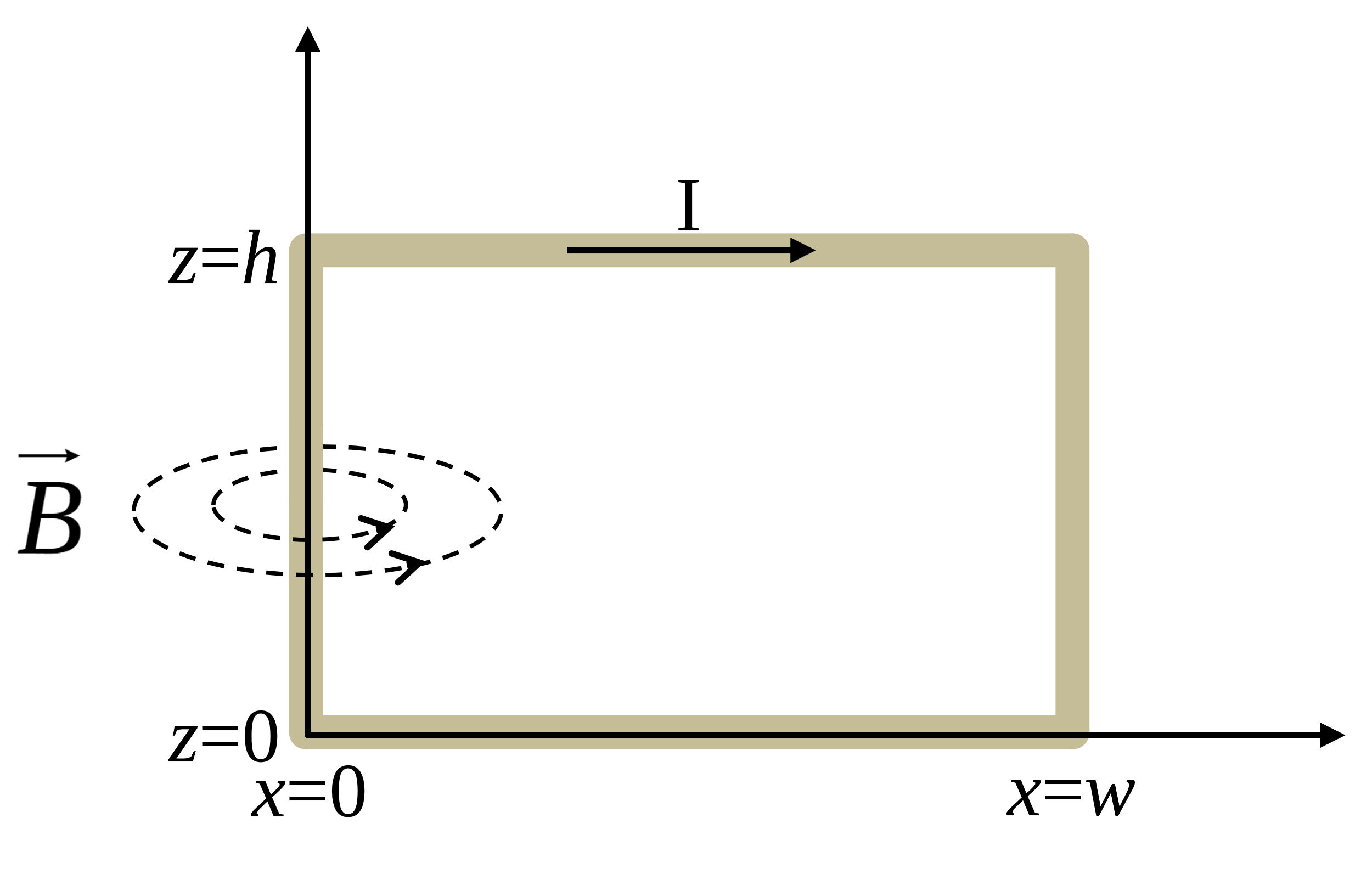
Place a uniform current, I, in the loop and calculate the total flux passing through the loop. For this example, it is convenient to start with the Biot-Savart Law, which expresses the H-field due to an incremental current element, I dl.

dH = I d × a ^ 12 4π R 12 2 A/m MathType@MTEF@5@5@+= feaahWart1ev3aqatCvAUfeBSjuyZL2yd9gzLbvyNv2CaerbpbxzUb YuH52CaeXatLxBI9gBaebbnrfifHhDYfgaruatPjwzYfgDP9MBGmvz YLMzaibaiKc9yrVq0xXdbba91rFfpec8Eeeu0xXdbba9frFj0=OqFf ea0dXdd9vqaq=JfrVkFHe9pgea0dXdar=Jb9hs0dXdbPYxe9vr0=vr 0=vqpWqaaeaabaGaaiaacaqabeaadaabamaaaOqaamaaFiaabaGaam izaiaadIeaaiaawEniaiabg2da9maalaaabaGaamysamaaFiaabaGa amizaiabjoriSbGaay51GaGaey41aq7aaecaaeaacaWGHbaacaGLcm aadaWgaaWcbaGaaGymaiaaikdaaeqaaaGcbaGaaGinaiabec8aWjaa dkfadaqhaaWcbaGaaGymaiaaikdaaeaacaaIYaaaaaaakiaaywW7ca qGbbGaae4laiaab2gacaaMe8oaaa@51AD@

where I is the amplitude of the current, R12 is the distance from the current element to the field point, and a ^ 12 MathType@MTEF@5@5@+= feaahWart1ev3aqatCvAUfeBSjuyZL2yd9gzLbvyNv2CaerbpbxzUb YuH52CaeXatLxBI9gBaebbnrfifHhDYfgaruatPjwzYfgDP9MBGmvz YLMzaibaiKc9yrVq0xXdbba91rFfpec8Eeeu0xXdbba9frFj0=OqFf ea0dXdd9vqaq=JfrVkFHe9pgea0dXdar=Jb9hs0dXdbPYxe9vr0=vr 0=vqpWqaaeaabaGaaiaacaqabeaadaabamaaaOqaamaaHaaabaGaam yyaaGaayPadaWaaSbaaSqaaiaaigdacaaIYaaabeaaaaa@3B35@ is a unit vector directed along the path of R12. To find the field at a point (r0,φ0,z0) due to the side of the rectangular loop located on the z axis in the figure, we make the substitution dl = zdz and integrate from z=0 to z=h,

H φ r 0 ,0, z 0 = 0 h I z ^ × a ^ 12 4π R 12 2 dzA/m. MathType@MTEF@5@5@+= feaahWart1ev3aqatCvAUfeBSjuyZL2yd9gzLbvyNv2CaerbpbxzUb YuH52CaeXatLxBI9gBaebbnrfifHhDYfgaruatPjwzYfgDP9MBGmvz YLMzaibaiKc9yrVq0xXdbba91rFfpec8Eeeu0xXdbba9frFj0=OqFf ea0dXdd9vqaq=JfrVkFHe9pgea0dXdar=Jb9hs0dXdbPYxe9vr0=vr 0=vqpWqaaeaabaGaaiaacaqabeaadaabamaaaOqaaiaadIeadaWgaa WcbaGaeqOXdOgabeaakmaabmaabaGaamOCamaaBaaaleaacaaIWaaa beaakiaacYcacaaIWaGaaiilaiaadQhadaWgaaWcbaGaaGimaaqaba aakiaawIcacaGLPaaacqGH9aqpdaWdXaqaamaalaaabaGaamysamaa bmaabaWaaecaaeaacaWG6baacaGLcmaacqGHxdaTdaqiaaqaaiaadg gaaiaawkWaamaaBaaaleaacaaIXaGaaGOmaaqabaaakiaawIcacaGL PaaaaeaacaaI0aGaeqiWdaNaamOuamaaDaaaleaacaaIXaGaaGOmaa qaaiaaikdaaaaaaaqaaiaaicdaaeaacaWGObaaniabgUIiYdGccaaM e8UaamizaiaadQhacaaMf8Uaaeyqaiaab+cacaqGTbGaaeOlaiaays W7aaa@5FE5@

For this problem, it is only necessary to solve for the φ component of H MathType@MTEF@5@5@+= feaahWart1ev3aqatCvAUfeBSjuyZL2yd9gzLbvyNv2CaerbpbxzUb YuH52CaeXatLxBI9gBaebbnrfifHhDYfgaruatPjwzYfgDP9MBGmvz YLMzaibaiKc9yrVq0xXdbba91rFfpec8Eeeu0xXdbba9frFj0=OqFf ea0dXdd9vqaq=JfrVkFHe9pgea0dXdar=Jb9hs0dXdbPYxe9vr0=vr 0=vqpWqaaeaabaGaaiaacaqabeaadaabamaaaOqaamaaFiaabaGaam isaaGaay51Gaaaaa@3A6B@ since this is the only component that penetrates the loop. Therefore, we are only interested in the radial component of a ^ 12 MathType@MTEF@5@5@+= feaahWart1ev3aqatCvAUfeBSjuyZL2yd9gzLbvyNv2CaerbpbxzUb YuH52CaeXatLxBI9gBaebbnrfifHhDYfgaruatPjwzYfgDP9MBGmvz YLMzaibaiKc9yrVq0xXdbba91rFfpec8Eeeu0xXdbba9frFj0=OqFf ea0dXdd9vqaq=JfrVkFHe9pgea0dXdar=Jb9hs0dXdbPYxe9vr0=vr 0=vqpWqaaeaabaGaaiaacaqabeaadaabamaaaOqaamaaHaaabaGaam yyaaGaayPadaWaaSbaaSqaaiaaigdacaaIYaaabeaaaaa@3B35@ , which is the cosine of the angle formed by the point (r,0,z0) and the z=0 plane. The cosine of this angle can be expressed as r 0 r 0 2 + z 0 2 MathType@MTEF@5@5@+= feaahWart1ev3aqatCvAUfeBSjuyZL2yd9gzLbvyNv2CaerbpbxzUb YuH52CaeXatLxBI9gBaebbnrfifHhDYfgaruatPjwzYfgDP9MBGmvz YLMzaibaiKc9yrVq0xXdbba91rFfpec8Eeeu0xXdbba9frFj0=OqFf ea0dXdd9vqaq=JfrVkFHe9pgea0dXdar=Jb9hs0dXdbPYxe9vr0=vr 0=vqpWqaaeaabaGaaiaacaqabeaadaabamaaaOqaamaalaaabaGaam OCamaaBaaaleaacaaIWaaabeaaaOqaamaakaaabaGaamOCamaaDaaa leaacaaIWaaabaGaaGOmaaaakiabgUcaRiaadQhadaqhaaWcbaGaaG imaaqaaiaaikdaaaaabeaaaaaaaa@4019@ . Therefore,

H φ r 0 ,0, z 0 = 0 h I r 0 4π r 0 2 + z z 0 2 3 2 dzA/m. MathType@MTEF@5@5@+= feaahWart1ev3aqatCvAUfeBSjuyZL2yd9gzLbvyNv2CaerbpbxzUb YuH52CaeXatLxBI9gBaebbnrfifHhDYfgaruatPjwzYfgDP9MBGmvz YLMzaibaiKc9yrVq0xXdbba91rFfpec8Eeeu0xXdbba9frFj0=OqFf ea0dXdd9vqaq=JfrVkFHe9pgea0dXdar=Jb9hs0dXdbPYxe9vr0=vr 0=vqpWqaaeaabaGaaiaacaqabeaadaabamaaaOqaaiaadIeadaWgaa WcbaGaeqOXdOgabeaakmaabmaabaGaamOCamaaBaaaleaacaaIWaaa beaakiaacYcacaaIWaGaaiilaiaadQhadaWgaaWcbaGaaGimaaqaba aakiaawIcacaGLPaaacqGH9aqpdaWdXaqaamaalaaabaGaamysaiaa ysW7caWGYbWaaSbaaSqaaiaaicdaaeqaaaGcbaGaaGinaiabec8aWn aadmaabaGaamOCamaaDaaaleaacaaIWaaabaGaaGOmaaaakiabgUca RmaabmaabaGaamOEaiabgkHiTiaadQhadaqhaaWcbaGaaGimaaqaaa aaaOGaayjkaiaawMcaamaaCaaaleqabaGaaGOmaaaaaOGaay5waiaa w2faamaaCaaaleqabaWaaSGaaeaacaaIZaaabaGaaGOmaaaaaaaaaa qaaiaaicdaaeaacaWGObaaniabgUIiYdGccaaMe8UaamizaiaadQha caaMf8Uaaeyqaiaab+cacaqGTbGaaeOlaiaaysW7aaa@64F4@

Performing the integration and multiplying by the permeability of free space, µ0, we obtain an expression for the φ-component of the magnetic flux density due to the first side of the loop,

B φ r 0 ,0, z 0 = μ 0 I 4π r 0 h z 0 r 0 2 + h z 0 2 + z 0 r 0 2 + z 0 2 Wb/m 2 . MathType@MTEF@5@5@+= feaahWart1ev3aqatCvAUfeBSjuyZL2yd9gzLbvyNv2CaerbpbxzUb YuH52CaeXatLxBI9gBaebbnrfifHhDYfgaruatPjwzYfgDP9MBGmvz YLMzaibaiKc9yrVq0xXdbba91rFfpec8Eeeu0xXdbba9frFj0=OqFf ea0dXdd9vqaq=JfrVkFHe9pgea0dXdar=Jb9hs0dXdbPYxe9vr0=vr 0=vqpWqaaeaabaGaaiaacaqabeaadaabamaaaOqaaiaadkeadaWgaa WcbaGaeqOXdOgabeaakmaabmaabaGaamOCamaaBaaaleaacaaIWaaa beaakiaacYcacaaIWaGaaiilaiaadQhadaWgaaWcbaGaaGimaaqaba aakiaawIcacaGLPaaacqGH9aqpdaWcaaqaaiabeY7aTnaaBaaaleaa caaIWaaabeaakiaadMeaaeaacaaI0aGaeqiWdaNaamOCamaaBaaale aacaaIWaaabeaaaaGcdaWadaqaamaalaaabaGaamiAaiabgkHiTiaa dQhadaWgaaWcbaGaaGimaaqabaaakeaadaGcaaqaaiaadkhadaqhaa WcbaGaaGimaaqaaiaaikdaaaGccqGHRaWkdaqadaqaaiaadIgacqGH sislcaWG6bWaaSbaaSqaaiaaicdaaeqaaaGccaGLOaGaayzkaaWaaW baaSqabeaacaaIYaaaaaqabaaaaOGaey4kaSYaaSaaaeaacaWG6bWa aSbaaSqaaiaaicdaaeqaaaGcbaWaaOaaaeaacaWGYbWaa0baaSqaai aaicdaaeaacaaIYaaaaOGaey4kaSIaamOEamaaDaaaleaacaaIWaaa baGaaGOmaaaaaeqaaaaaaOGaay5waiaaw2faaiaaywW7caqGxbGaae Oyaiaab+cacaqGTbWaaWbaaSqabeaacaqGYaaaaOGaaiOlaiaaysW7 aaa@6BEC@

To find the total flux penetrating the loop due to this segment, we integrate the flux density over the loop area, assuming that the wire radius is much smaller than the height and width of the loop.

ψ side1 a w 0 h B φ r 0 ,0, z 0 dzdr a w μ 0 I 4π r 0 0 h h z 0 r 0 2 + h z 0 2 + z 0 r 0 2 + z 0 2 dzdr a w μ 0 I 4π r 0 2r+ 2 h 2 + r 2 r dr μ 0 I 2π aw+ h 2 + w 2 hln h+ h 2 + w 2 w h+hln 2h a μ 0 I 2π w+ h 2 + w 2 hln h+ h 2 + w 2 w h+hln 2h a webers. MathType@MTEF@5@5@+= feaahWart1ev3aqatCvAUfeBSjuyZL2yd9gzLbvyNv2CaerbpbxzUb YuH52CaeXatLxBI9gBaebbnrfifHhDYfgaruatPjwzYfgDP9MBGmvz YLMzaibaiKc9yrVq0xXdbba91rFfpec8Eeeu0xXdbba9frFj0=OqFf ea0dXdd9vqaq=JfrVkFHe9pgea0dXdar=Jb9hs0dXdbPYxe9vr0=vr 0=vqpWqaaeaabaGaaiaacaqabeaadaabamaaaOabaqqabaGaeqiYdK 3aaSbaaSqaaiaadohacaWGPbGaamizaiaadwgacaaIXaaabeaakiab gIKi7oaapedabaWaa8qmaeaacaWGcbWaaSbaaSqaaiabeA8aQbqaba GcdaqadaqaaiaadkhadaWgaaWcbaGaaGimaaqabaGccaGGSaGaaGim aiaacYcacaWG6bWaaSbaaSqaaiaaicdaaeqaaaGccaGLOaGaayzkaa GaaGjbVlaadsgacaWG6bGaaGPaVlaadsgacaWGYbaaleaacaaIWaaa baGaamiAaaqdcqGHRiI8aaWcbaGaamyyaaqaaiaadEhaa0Gaey4kIi paaOqaaiabgIKi7oaapedabaWaaSaaaeaacqaH8oqBdaWgaaWcbaGa aGimaaqabaGccaWGjbaabaGaaGinaiabec8aWjaadkhadaWgaaWcba GaaGimaaqabaaaaOWaa8qmaeaadaWadaqaamaalaaabaGaamiAaiab gkHiTiaadQhadaWgaaWcbaGaaGimaaqabaaakeaadaGcaaqaaiaadk hadaqhaaWcbaGaaGimaaqaaiaaikdaaaGccqGHRaWkdaqadaqaaiaa dIgacqGHsislcaWG6bWaaSbaaSqaaiaaicdaaeqaaaGccaGLOaGaay zkaaWaaWbaaSqabeaacaaIYaaaaaqabaaaaOGaey4kaSYaaSaaaeaa caWG6bWaaSbaaSqaaiaaicdaaeqaaaGcbaWaaOaaaeaacaWGYbWaa0 baaSqaaiaaicdaaeaacaaIYaaaaOGaey4kaSIaamOEamaaDaaaleaa caaIWaaabaGaaGOmaaaaaeqaaaaaaOGaay5waiaaw2faaaWcbaGaaG imaaqaaiaadIgaa0Gaey4kIipakiaaysW7caWGKbGaamOEaiaaysW7 caWGKbGaamOCaaWcbaGaamyyaaqaaiaadEhaa0Gaey4kIipaaOqaai abgIKi7oaapedabaWaaSaaaeaacqaH8oqBdaWgaaWcbaGaaGimaaqa baGccaWGjbaabaGaaGinaiabec8aWjaadkhadaWgaaWcbaGaaGimaa qabaaaaOWaamWaaeaacqGHsislcaaIYaGaamOCaiabgUcaRmaalaaa baGaaGOmamaakaaabaGaamiAamaaCaaaleqabaGaaGOmaaaakiabgU caRiaadkhadaahaaWcbeqaaiaaikdaaaaabeaaaOqaaiaadkhaaaaa caGLBbGaayzxaaGaamizaiaadkhaaSqaaiaadggaaeaacaWG3baani abgUIiYdaakeaacqGHijYUdaWcaaqaaiabeY7aTnaaBaaaleaacaaI WaaabeaakiaadMeaaeaacaaIYaGaeqiWdahaamaadmaabaGaamyyai abgkHiTiaadEhacqGHRaWkdaGcaaqaaiaadIgadaahaaWcbeqaaiaa ikdaaaGccqGHRaWkcaWG3bWaaWbaaSqabeaacaaIYaaaaaqabaGccq GHsislcaWGObGaaGPaVlGacYgacaGGUbWaaeWaaeaadaWcaaqaaiaa dIgacqGHRaWkdaGcaaqaaiaadIgadaahaaWcbeqaaiaaikdaaaGccq GHRaWkcaWG3bWaaWbaaSqabeaacaaIYaaaaaqabaaakeaacaWG3baa aaGaayjkaiaawMcaaiabgkHiTiaadIgacqGHRaWkcaWGObGaaGPaVl GacYgacaGGUbWaaeWaaeaadaWcaaqaaiaaikdacaWGObaabaGaamyy aaaaaiaawIcacaGLPaaaaiaawUfacaGLDbaaaeaacqGHijYUdaWcaa qaaiabeY7aTnaaBaaaleaacaaIWaaabeaakiaadMeaaeaacaaIYaGa eqiWdahaamaadmaabaGaeyOeI0Iaam4DaiabgUcaRmaakaaabaGaam iAamaaCaaaleqabaGaaGOmaaaakiabgUcaRiaadEhadaahaaWcbeqa aiaaikdaaaaabeaakiabgkHiTiaadIgacaaMc8UaciiBaiaac6gada qadaqaamaalaaabaGaamiAaiabgUcaRmaakaaabaGaamiAamaaCaaa leqabaGaaGOmaaaakiabgUcaRiaadEhadaahaaWcbeqaaiaaikdaaa aabeaaaOqaaiaadEhaaaaacaGLOaGaayzkaaGaeyOeI0IaamiAaiab gUcaRiaadIgacaaMc8UaciiBaiaac6gadaqadaqaamaalaaabaGaaG OmaiaadIgaaeaacaWGHbaaaaGaayjkaiaawMcaaaGaay5waiaaw2fa aiaaysW7caqG3bGaaeyzaiaabkgacaqGLbGaaeOCaiaabohacaqGUa aaaaa@043A@

By symmetry, the total flux coupling the loop due to the segment on the opposite side of the loop is the same. An expression for the total flux coupling the loop due to the top and bottom segments is obtained by interchanging the w and h in the equation above. Summing the flux contributions from all four sides and dividing by the current gives an expression for the self-inductance of the loop,

L rect loop μ 0 π 2 w+h +2 h 2 + w 2 hln h+ h 2 + w 2 w wln w+ h 2 + w 2 h +hln 2h a +wln 2w a henries. MathType@MTEF@5@5@+= feaahWart1ev3aqatCvAUfeBSjuyZL2yd9gzLbvyNv2CaerbpbxzUb YuH52CaeXatLxBI9gBaebbnrfifHhDYfgaruatPjwzYfgDP9MBGmvz YLMzaibaiKc9yrVq0xXdbba91rFfpec8Eeeu0xXdbba9frFj0=OqFf ea0dXdd9vqaq=JfrVkFHe9pgea0dXdar=Jb9hs0dXdbPYxe9vr0=vr 0=vqpWqaaeaabaGaaiaacaqabeaadaabamaaaOabaeqabaGaamitam aaBaaaleaacaqGYbGaaeyzaiaabogacaqG0bGaaeiiaiaabYgacaqG VbGaae4BaiaabchaaeqaaOGaeyisIS7aaSaaaeaacqaH8oqBdaWgaa WcbaGaaGimaaqabaaakeaacqaHapaCaaWaamqaaeaacqGHsislcaaI YaWaaeWaaeaacaWG3bGaey4kaSIaamiAaaGaayjkaiaawMcaaiabgU caRiaaikdadaGcaaqaaiaadIgadaahaaWcbeqaaiaaikdaaaGccqGH RaWkcaWG3bWaaWbaaSqabeaacaaIYaaaaaqabaaakiaawUfaaiabgk HiTiaadIgacaaMc8UaciiBaiaac6gadaqadaqaamaalaaabaGaamiA aiabgUcaRmaakaaabaGaamiAamaaCaaaleqabaGaaGOmaaaakiabgU caRiaadEhadaahaaWcbeqaaiaaikdaaaaabeaaaOqaaiaadEhaaaaa caGLOaGaayzkaaaabaGaaGzbVlaaywW7caaMf8UaaGzbVlaaywW7ca aMf8UaaGzbVpaadiaabaGaeyOeI0Iaam4DaiaaykW7ciGGSbGaaiOB amaabmaabaWaaSaaaeaacaWG3bGaey4kaSYaaOaaaeaacaWGObWaaW baaSqabeaacaaIYaaaaOGaey4kaSIaam4DamaaCaaaleqabaGaaGOm aaaaaeqaaaGcbaGaamiAaaaaaiaawIcacaGLPaaacqGHRaWkcaWGOb GaaGPaVlGacYgacaGGUbWaaeWaaeaadaWcaaqaaiaaikdacaWGObaa baGaamyyaaaaaiaawIcacaGLPaaacqGHRaWkcaWG3bGaaGPaVlGacY gacaGGUbWaaeWaaeaadaWcaaqaaiaaikdacaWG3baabaGaamyyaaaa aiaawIcacaGLPaaaaiaaw2faaiaaykW7caaMc8UaaeiAaiaabwgaca qGUbGaaeOCaiaabMgacaqGLbGaae4Caiaab6cacaaMe8oaaaa@9C22@

Although this is a simple loop, the closed-form solution for the inductance is not a simple expression. To make things a little more intuitive, we can consider the case where h=w (i.e., a square loop),

(3)

L square loop 2 μ 0 w π ln w a 0.774 MathType@MTEF@5@5@+= feaahWart1ev3aqatCvAUfeBSjuyZL2yd9gzLbvyNv2CaerbpbxzUb YuH52CaeXatLxBI9gBaebbnrfifHhDYfgaruatPjwzYfgDP9MBGmvz YLMzaibaiKc9yrVq0xXdbba91rFfpec8Eeeu0xXdbba9frFj0=OqFf ea0dXdd9vqaq=JfrVkFHe9pgea0dXdar=Jb9hs0dXdbPYxe9vr0=vr 0=vqpWqaaeaabaGaaiaacaqabeaadaabamaaaOqaaiaadYeadaWgaa WcbaGaam4CaiaadghacaWG1bGaamyyaiaadkhacaWGLbGaaeiiaiaa dYgacaWGVbGaam4BaiaadchaaeqaaOGaeyisIS7aaSaaaeaacaaIYa GaeqiVd02aaSbaaSqaaiaaicdaaeqaaOGaam4Daaqaaiabec8aWbaa daWadaqaaiGacYgacaGGUbWaaeWaaeaadaWcaaqaaiaadEhaaeaaca WGHbaaaaGaayjkaiaawMcaaiabgkHiTiaaicdacaGGUaGaaG4naiaa iEdacaaI0aaacaGLBbGaayzxaaaaaa@56D7@ henries.

The size of the loop is the most important parameter affecting the inductance. For >> a, the inductance is proportional to [(ln w)]. It is not proportional to the loop area, w2, but loops with larger loop areas tend to have higher inductances. The wire diameter also plays a role, especially for very thin wires. Note that a loop constructed of infinitely thin wire would have infinite inductance.

In the example above, we began integrating at the wire surface (r = a). In other words, we neglected any magnetic flux that may have existed within the wire itself. Inductance calculated using only the loop area external to the wire surface is called external inductance. At high frequencies, where the skin depth is a fraction of the wire diameter, most of the current flows near the surface of the wire and the flux inside the wire is nearly zero. In this case, the total inductance is essentially equal to the external inductance.

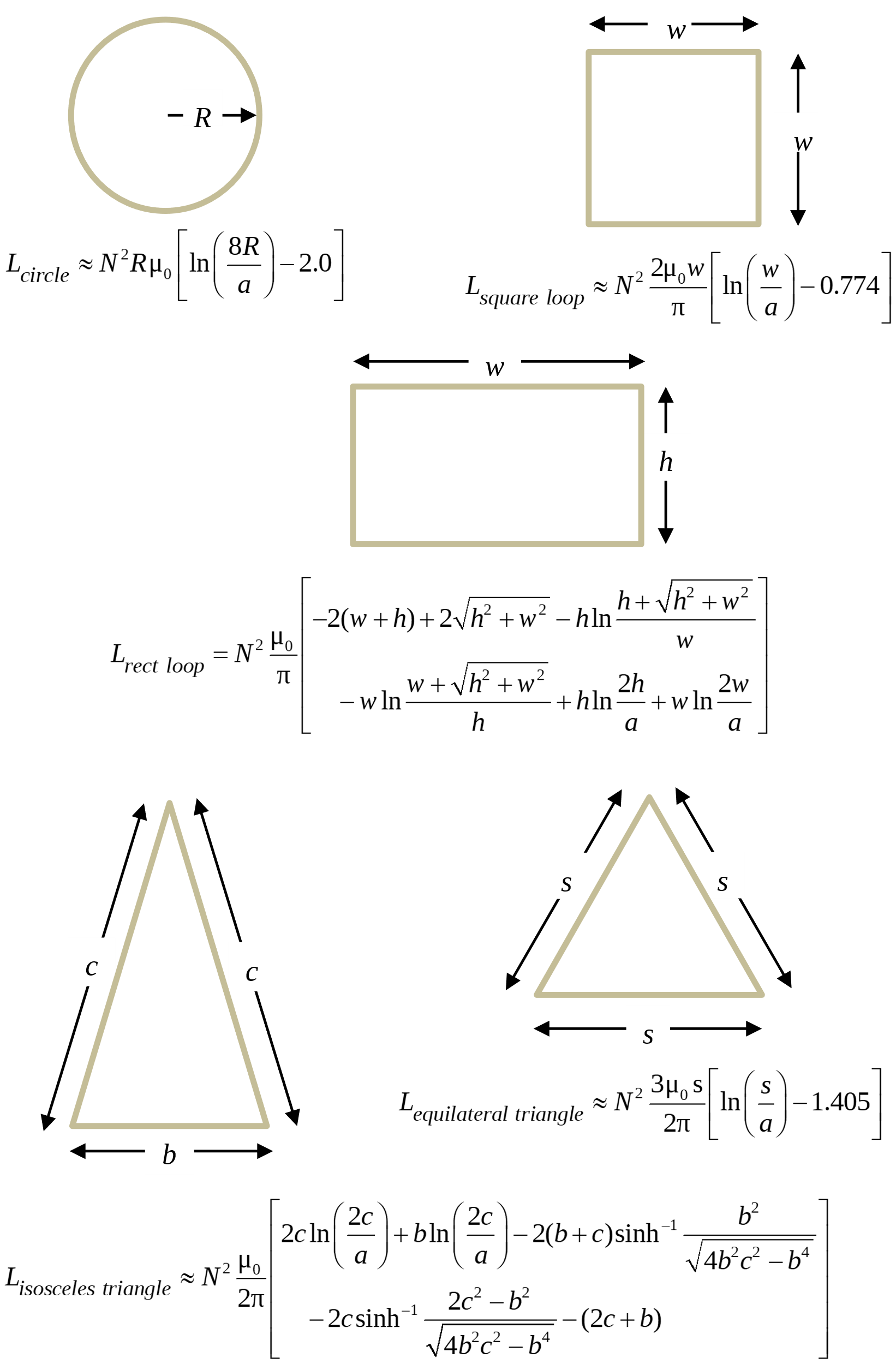
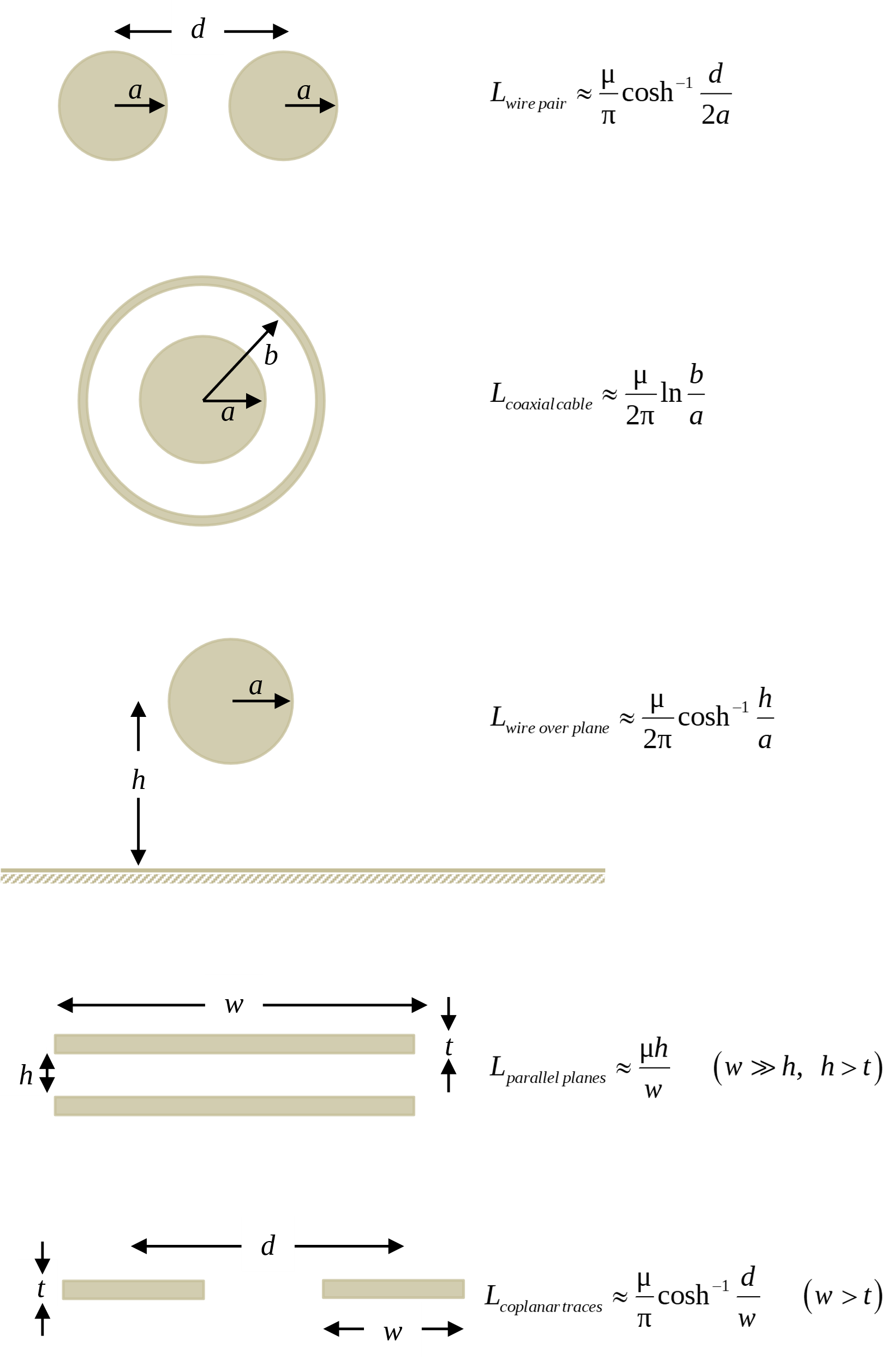
Figure 2 provides closed-form expressions for the external self-inductance of five wire-loop geometries. For transmission line geometries that are much longer in one dimension than the other two, it is generally more accurate to calculate the inductance per unit length using the equations in Figure 3. The overall inductance of the loop can then be calculated by multiplying the inductance per unit length by the length of the transmission line.

Internal Inductance

At low frequencies where the diameter of a wire is less than a skin depth, the current distribution within the wire is nearly uniform. This means that magnetic flux within the wire couples the loop and contributes to the overall inductance. Calculating the exact contribution of this internal flux can be complicated because both the amount of flux and the loop area are functions of position within the wire. However, for wires with a circular cross-section, an expression for the internal inductance per unit length can be derived based on an energy definition of inductance (see Example 2).

At high frequencies, where inductance is most likely to be a concern, the internal inductance approaches zero due to the skin effect. At low frequencies, the total inductance is the sum of the internal and external inductances. In most circuits, the internal inductance at any frequency contributes little to the overall loop inductance. While it’s important to be familiar with the concept of internal inductance, this inductance can often be neglected when solving for the self-inductance of practical configurations.

External inductance of round wire loop geometries

Figure 2. External inductance of round wire loop geometries
(wire radius = a, number of turns = N).

 
External inductance per unit length of transmission line geometries
Figure 3. External inductance per unit length of transmission line geometries.
 

Example 2: Internal Inductance of a Round Wire

The energy stored in an inductance is equal to ½ LI². The energy stored in a magnetic field is equal to the energy density of the field, ½ µ|H|2, integrated over the entire volume of the field. Using these expressions, we can equate the energy stored by the internal inductance of a wire to the energy stored in the magnetic field within a wire that has a circular cross-section,

1 2 L wire-internal I 2 = v μ 2 H 2 dv(Joules) = μ 2 0 0 2π 0 a Ir 2π a 2 2 rdrdφdz MathType@MTEF@5@5@+= feaahWart1ev3aqatCvAUfeBSjuyZL2yd9gzLbvyNv2CaerbpbxzUb YuH52CaeXatLxBI9gBaebbnrfifHhDYfgaruatPjwzYfgDP9MBGmvz YLMzaibaiKc9yrVq0xXdbba91rFfpec8Eeeu0xXdbba9frFj0=OqFf ea0dXdd9vqaq=JfrVkFHe9pgea0dXdar=Jb9hs0dXdbPYxe9vr0=vr 0=vqpWqaaeaabaGaaiaacaqabeaadaabamaaaOabaqqabaWaaSaaae aacaaIXaaabaGaaGOmaaaacaWGmbWaaSbaaSqaaiaabEhacaqGPbGa aeOCaiaabwgacaqGTaGaaeyAaiaab6gacaqG0bGaaeyzaiaabkhaca qGUbGaaeyyaiaabYgaaeqaaOGaaGjbVlaadMeadaahaaWcbeqaaiaa ikdaaaGccqGH9aqpdaWdrbqaamaalaaabaGaeqiVd0gabaGaaGOmaa aaaSqaaiaadAhaaeqaniabgUIiYdGcdaabdaqaamaaFiaabaGaamis aaGaay51GaaacaGLhWUaayjcSdWaaWbaaSqabeaacaaIYaaaaOGaaG jbVlaadsgacaWG2bGaaGzbVlaabIcacaqGkbGaae4BaiaabwhacaqG SbGaaeyzaiaabohacaqGPaaabaGaeyypa0ZaaSaaaeaacqaH8oqBae aacaaIYaaaamaapedabaWaa8qmaeaadaWdXaqaamaaemaabaWaaSaa aeaacaWGjbGaamOCaiaaysW7aeaacaaIYaGaeqiWdaNaamyyamaaCa aaleqabaGaaGOmaaaaaaaakiaawEa7caGLiWoaaSqaaiaaicdaaeaa caWGHbaaniabgUIiYdaaleaacaaIWaaabaGaaGOmaiabec8aWbqdcq GHRiI8aaWcbaGaaGimaaqaaiabjoriSbqdcqGHRiI8aOWaaWbaaSqa beaacaaIYaaaaOGaaGPaVlaadkhacaaMc8UaamizaiaadkhacaaMc8 UaamizaiabeA8aQjaaykW7caWGKbGaamOEaiaaysW7aaaa@8EAF@

where µ is the permeability of the wire and l is the length of the wire.

Solving for Lwire-internal, we obtain,

L wire-internal = μ 8π henries. MathType@MTEF@5@5@+= feaahWart1ev3aqatCvAUfeBSjuyZL2yd9gzLbvyNv2CaerbpbxzUb YuH52CaeXatLxBI9gBaebbnrfifHhDYfgaruatPjwzYfgDP9MBGmvz YLMzaibaiKc9yrVq0xXdbba91rFfpec8Eeeu0xXdbba9frFj0=OqFf ea0dXdd9vqaq=JfrVkFHe9pgea0dXdar=Jb9hs0dXdbPYxe9vr0=vr 0=vqpWqaaeaabaGaaiaacaqabeaadaabamaaaOqaaiaadYeadaWgaa WcbaGaae4DaiaabMgacaqGYbGaaeyzaiaab2cacaqGPbGaaeOBaiaa bshacaqGLbGaaeOCaiaab6gacaqGHbGaaeiBaaqabaGccaaMe8Uaey ypa0ZaaSaaaeaacqaH8oqBaeaacaaI4aGaeqiWdahaaiabjoriSjaa ywW7caqGObGaaeyzaiaab6gacaqGYbGaaeyAaiaabwgacaqGZbGaae Olaaaa@55A2@

Note that the expression for the internal inductance of a round wire is independent of the radius of the wire. For copper or aluminum wires, µ = µ0 and the internal inductance per unit length is approximately µ0/8π or 50 nH/m.

Mutual Inductance

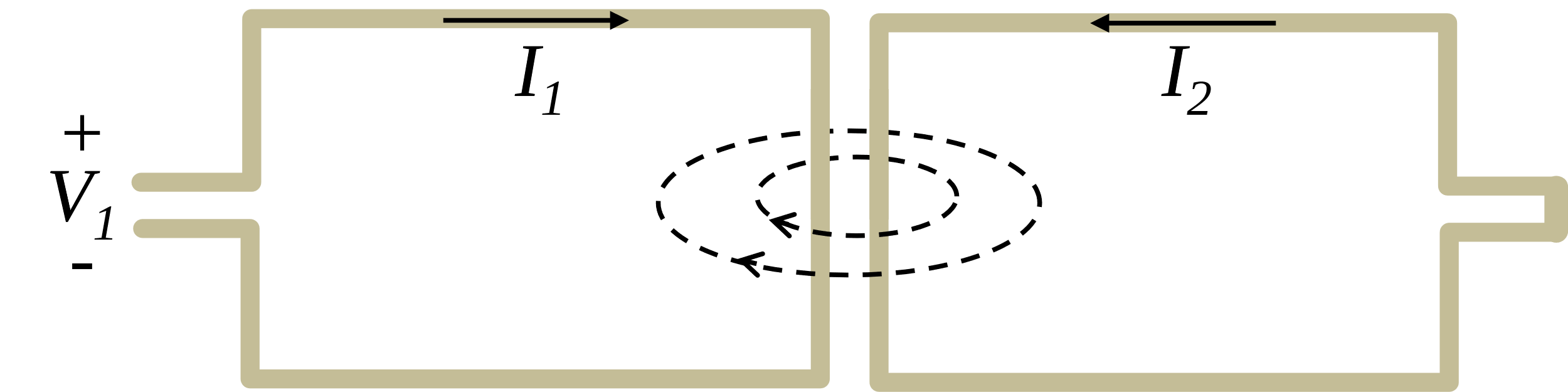
Just as two conducting objects can have a mutual capacitance, two current loops can have a mutual inductance. Figure 4 illustrates the concept of mutual inductance. Two wire loops are shown. A current in the first loop generates a magnetic flux. Some of this flux passes through (or links) the second loop. The mutual inductance is defined as the ratio of the total magnetic flux that links the second loop divided by the current in the first loop,

(4)

L 21 = Ψ 21 I 1 MathType@MTEF@5@5@+= feaahWart1ev3aqatCvAUfeBSjuyZL2yd9gzLbvyNv2CaerbpbxzUb YuH52CaeXatLxBI9gBaebbnrfifHhDYfgaruatPjwzYfgDP9MBGmvz YLMzaibaiKc9yrVq0xXdbba91rFfpec8Eeeu0xXdbba9frFj0=OqFf ea0dXdd9vqaq=JfrVkFHe9pgea0dXdar=Jb9hs0dXdbPYxe9vr0=vr 0=vqpWqaaeaabaGaaiaacaqabeaadaabamaaaOqaaiaadYeadaWgaa WcbaGaaGOmaiaaigdaaeqaaOGaeyypa0ZaaSaaaeaacqqHOoqwdaWg aaWcbaGaaGOmaiaaigdaaeqaaaGcbaGaamysamaaBaaaleaacaaIXa aabeaaaaaaaa@406F@ henries.

Figure 4. Mutual inductance in a pair of current loops.

If loop 2 consists of a single turn of wire (i.e., no flux lines can pass through the loop twice), then Ψ21 must be some fraction of the total flux generated by loop 1, Ψ11.

The coupled flux, Ψ21, can be written as the integral of the coupled flux density over the surface of the second loop,

(5)

L 21 = S2 B 1 ds I 1 MathType@MTEF@5@5@+= feaahWart1ev3aqatCvAUfeBSjuyZL2yd9gzLbvyNv2CaerbpbxzUb YuH52CaeXatLxBI9gBaebbnrfifHhDYfgaruatPjwzYfgDP9MBGmvz YLMzaibaiKc9yrVq0xXdbba91rFfpec8Eeeu0xXdbba9frFj0=OqFf ea0dXdd9vqaq=JfrVkFHe9pgea0dXdar=Jb9hs0dXdbPYxe9vr0=vr 0=vqpWqaaeaabaGaaiaacaqabeaadaabamaaaOqaaiaadYeadaWgaa WcbaGaaGOmaiaaigdaaeqaaOGaeyypa0ZaaSaaaeaadaWdraqaamaa FiaabaGaamOqaaGaay51GaWaaSbaaSqaaiaaigdaaeqaaOGaeyyXIC 9aa8HaaeaacaWGKbGaam4CaaGaay51GaaaleaacaWGtbGaaGOmaaqa b0Gaey4kIipaaOqaaiaadMeadaWgaaWcbaGaaGymaaqabaaaaaaa@4A26@ henries.

Applying Stokes’s theorem, we can convert the surface integral above to a line integral,

(6)

L 21 = S2 × A 1 ds I 1 = A 1 dl 2 I 1 MathType@MTEF@5@5@+= feaahWart1ev3aqatCvAUfeBSjuyZL2yd9gzLbvyNv2CaerbpbxzUb YuH52CaeXatLxBI9gBaebbnrfifHhDYfgaruatPjwzYfgDP9MBGmvz YLMzaibaiKc9yrVq0xXdbba91rFfpec8Eeeu0xXdbba9frFj0=OqFf ea0dXdd9vqaq=JfrVkFHe9pgea0dXdar=Jb9hs0dXdbPYxe9vr0=vr 0=vqpWqaaeaabaGaaiaacaqabeaadaabamaaaOqaaiaadYeadaWgaa WcbaGaaGOmaiaaigdaaeqaaOGaeyypa0ZaaSaaaeaadaWdrbqaamaa bmaabaGaey4bIeTaey41aq7aa8HaaeaacaWGbbaacaGLxdcadaWgaa WcbaGaaGymaaqabaaakiaawIcacaGLPaaacqGHflY1daWhcaqaaiaa dsgacaWGZbaacaGLxdcaaSqaaiaadofacaaIYaaabeqdcqGHRiI8aa GcbaGaamysamaaBaaaleaacaaIXaaabeaaaaGccqGH9aqpdaWcaaqa amaapuaabaWaa8HaaeaacaWGbbaacaGLxdcadaWgaaWcbaGaaGymaa qabaGccqGHflY1daWhcaqaaiaadsgacqa6tecBaiaawEniamaaBaaa leaacaaIYaaabeaaaeqabeqdcqWIr4E0cqGHRiI8aaGcbaGaamysam aaBaaaleaacaaIXaaabeaaaaaaaa@6187@ henries

where A 1 MathType@MTEF@5@5@+= feaahWart1ev3aqatCvAUfeBSjuyZL2yd9gzLbvyNv2CaerbpbxzUb YuH52CaeXatLxBI9gBaebbnrfifHhDYfgaruatPjwzYfgDP9MBGmvz YLMzaibaiKc9yrVq0xXdbba91rFfpec8Eeeu0xXdbba9frFj0=OqFf ea0dXdd9vqaq=JfrVkFHe9pgea0dXdar=Jb9hs0dXdbPYxe9vr0=vr 0=vqpWqaaeaabaGaaiaacaqabeaadaabamaaaOqaamaaFiaabaGaam yqaaGaay51GaWaaSbaaSqaaiaaigdaaeqaaaaa@3B4B@ is the magnetic vector potential due to the current in the first loop. This vector potential can be expressed as a function of the current in this loop,

(7)

A 1 = μ I 1 4πR d MathType@MTEF@5@5@+= feaahWart1ev3aqatCvAUfeBSjuyZL2yd9gzLbvyNv2CaerbpbxzUb YuH52CaeXatLxBI9gBaebbnrfifHhDYfgaruatPjwzYfgDP9MBGmvz YLMzaibaiKc9yrVq0xXdbba91rFfpec8Eeeu0xXdbba9frFj0=OqFf ea0dXdd9vqaq=JfrVkFHe9pgea0dXdar=Jb9hs0dXdbPYxe9vr0=vr 0=vqpWqaaeaabaGaaiaacaqabeaadaabamaaaOqaamaaFiaabaGaam yqaaGaay51GaWaaSbaaSqaaiaaigdaaeqaaOGaeyypa0Zaa8qbaeaa daWcaaqaaiabeY7aTjaadMeadaWgaaWcbaGaaGymaaqabaaakeaaca aI0aGaeqiWdaNaamOuaaaaaSqabeqaniablgH7rlabgUIiYdGccaaM e8+aa8HaaeaacaWGKbGaeK4eHWgacaGLxdcaaaa@4CF5@ webers/m

where R is the distance between the current element, dl, and the field point. Combining Equations (6) and (7), we get an expression for the mutual inductance that is independent of the current,

(8)

L 21 = μ 4π d 1 d 2 R MathType@MTEF@5@5@+= feaahWart1ev3aqatCvAUfeBSjuyZL2yd9gzLbvyNv2CaerbpbxzUb YuH52CaeXatLxBI9gBaebbnrfifHhDYfgaruatPjwzYfgDP9MBGmvz YLMzaibaiKc9yrVq0xXdbba91rFfpec8Eeeu0xXdbba9frFj0=OqFf ea0dXdd9vqaq=JfrVkFHe9pgea0dXdar=Jb9hs0dXdbPYxe9vr0=vr 0=vqpWqaaeaabaGaaiaacaqabeaadaabamaaaOqaaiaadYeadaWgaa WcbaGaaGOmaiaaigdaaeqaaOGaeyypa0ZaaSaaaeaacqaH8oqBaeaa caaI0aGaeqiWdahaamaapuaabaWaa8qbaeaadaWcaaqaamaaFiaaba GaamizaiabjoriSbGaay51GaWaaSbaaSqaaiaaigdaaeqaaOGaeyyX IC9aa8HaaeaacaWGKbGaeK4eHWgacaGLxdcadaWgaaWcbaGaaGOmaa qabaaakeaacaWGsbaaaaWcbeqab0GaeSyeUhTaey4kIipaaSqabeqa niablgH7rlabgUIiYdaaaa@551B@ henries.

It is clear from this expression that L21 = L12 since the integration in the loops can be taken in either order.

Another useful expression for the mutual inductance between two loops with self-inductances, L11 and L22, is

(9)

L 21 =k L 11 L 22 MathType@MTEF@5@5@+= feaahWart1ev3aqatCvAUfeBSjuyZL2yd9gzLbvyNv2CaerbpbxzUb YuH52CaeXatLxBI9gBaebbnrfifHhDYfgaruatPjwzYfgDP9MBGmvz YLMzaibaiKc9yrVq0xXdbba91rFfpec8Eeeu0xXdbba9frFj0=OqFf ea0dXdd9vqaq=JfrVkFHe9pgea0dXdar=Jb9hs0dXdbPYxe9vr0=vr 0=vqpWqaaeaabaGaaiaacaqabeaadaabamaaaOqaaiaadYeadaWgaa WcbaGaaGOmaiaaigdaaeqaaOGaeyypa0Jaam4AamaakaaabaGaamit amaaBaaaleaacaaIXaGaaGymaaqabaGccaWGmbWaaSbaaSqaaiaaik dacaaIYaaabeaaaeqaaaaa@4160@ henries

where 0 ≤ k < 1 depends on the fraction of the total flux that couples both loops. From this expression, it is clear that the mutual inductance cannot exceed the self-inductance of the larger loop.

Effective Inductance

The term effective inductance is often used to describe the inductance that would be measured between two terminals in a system. If the measured impedance across these terminals is a positive reactance (i.e., imaginary and positive) at one particular frequency, it looks like an inductance. If the measured impedance is also proportional to frequency over a given frequency range, the inductance is constant over that entire range of frequencies.

Example 3: Effective Inductance of a Pair of Circuits

The two wire loops illustrated below have a self-inductance of 100 nH. The mutual inductance between the two loops is 20 nH. What is the effective inductance as viewed from the input terminals of the first loop?

We can start by defining the voltage and current in the first loop as V1 and I1, respectively. The voltage and current in the second loop are V2 and I2, and we can write the system of equations for the voltages and currents as follows,

V 1 =jω L 11 I 1 ±jω L 12 I 2 MathType@MTEF@5@5@+= feaahWart1ev3aqatCvAUfeBSjuyZL2yd9gzLbvyNv2CaerbpbxzUb YuH52CaeXatLxBI9gBaebbnrfifHhDYfgaruatPjwzYfgDP9MBGmvz YLMzaibaiKc9yrVq0xXdbba91rFfpec8Eeeu0xXdbba9frFj0=OqFf ea0dXdd9vqaq=JfrVkFHe9pgea0dXdar=Jb9hs0dXdbPYxe9vr0=vr 0=vqpWqaaeaabaGaaiaacaqabeaadaabamaaaOqaaiaadAfadaWgaa WcbaGaaGymaaqabaGccqGH9aqpcaWGQbGaeqyYdCNaaGjcVlaadYea daWgaaWcbaGaaGymaiaaigdaaeqaaOGaamysamaaBaaaleaacaaIXa aabeaakiabgglaXkaadQgacqaHjpWDcaaMi8UaamitamaaBaaaleaa caaIXaGaaGOmaaqabaGccaWGjbWaaSbaaSqaaiaaikdaaeqaaaaa@4DB4@

V 2 =jω L 21 I 1 ±jω L 22 I 2 MathType@MTEF@5@5@+= feaahWart1ev3aqatCvAUfeBSjuyZL2yd9gzLbvyNv2CaerbpbxzUb YuH52CaeXatLxBI9gBaebbnrfifHhDYfgaruatPjwzYfgDP9MBGmvz YLMzaibaiKc9yrVq0xXdbba91rFfpec8Eeeu0xXdbba9frFj0=OqFf ea0dXdd9vqaq=JfrVkFHe9pgea0dXdar=Jb9hs0dXdbPYxe9vr0=vr 0=vqpWqaaeaabaGaaiaacaqabeaadaabamaaaOqaaiaadAfadaWgaa WcbaGaaGOmaaqabaGccqGH9aqpcaWGQbGaeqyYdCNaaGjcVlaadYea daWgaaWcbaGaaGOmaiaaigdaaeqaaOGaamysamaaBaaaleaacaaIXa aabeaakiabgglaXkaadQgacqaHjpWDcaaMi8UaamitamaaBaaaleaa caaIYaGaaGOmaaqabaGccaWGjbWaaSbaaSqaaiaaikdaaeqaaaaa@4DB7@

The ± in these equations indicates that the flux generated by a current in Loop 2 can either add to or subtract from the flux generated by the current in Loop 1, depending on the orientation of the loops. In this case, the current induced in Loop 2 by the current in Loop 1 will generate a flux that opposes the flux in Loop 1, so the minus sign is the correct choice.

Since the second loop is shorted, V2 = 0, and substituting into the second equation above yields,

I 2 = L 21 L 22 I 1 = 20nH 100nH I 1 =0.20 I 1 MathType@MTEF@5@5@+= feaahWart1ev3aqatCvAUfeBSjuyZL2yd9gzLbvyNv2CaerbpbxzUb YuH52CaeXatLxBI9gBaebbnrfifHhDYfgaruatPjwzYfgDP9MBGmvz YLMzaibaiKc9yrVq0xXdbba91rFfpec8Eeeu0xXdbba9frFj0=OqFf ea0dXdd9vqaq=JfrVkFHe9pgea0dXdar=Jb9hs0dXdbPYxe9vr0=vr 0=vqpWqaaeaabaGaaiaacaqabeaadaabamaaaOqaaiaadMeadaWgaa WcbaGaaGOmaaqabaGccqGH9aqpdaWcaaqaaiaadYeadaWgaaWcbaGa aGOmaiaaigdaaeqaaaGcbaGaamitamaaBaaaleaacaaIYaGaaGOmaa qabaaaaOGaamysamaaBaaaleaacaaIXaaabeaakiabg2da9maalaaa baGaaGOmaiaaicdacaaMe8UaaeOBaiaabIeaaeaacaaIXaGaaGimai aaicdacaaMe8UaaeOBaiaabIeaaaGaamysamaaBaaaleaacaaIXaaa beaakiabg2da9iaaicdacaGGUaGaaGOmaiaaicdacaWGjbWaaSbaaS qaaiaaigdaaeqaaaaa@5425@

Therefore, the equation above for V1 can be rewritten,

V 1 =jω 100nH I 1 jω 20nH 0.2 I 1 =jω 96nH I 1 . MathType@MTEF@5@5@+= feaahWart1ev3aqatCvAUfeBSjuyZL2yd9gzLbvyNv2CaerbpbxzUb YuH52CaeXatLxBI9gBaebbnrfifHhDYfgaruatPjwzYfgDP9MBGmvz YLMzaibaiKc9yrVq0xXdbba91rFfpec8Eeeu0xXdbba9frFj0=OqFf ea0dXdd9vqaq=JfrVkFHe9pgea0dXdar=Jb9hs0dXdbPYxe9vr0=vr 0=vqpWqaaeaabaGaaiaacaqabeaadaabamaaaOqaaiaadAfadaWgaa WcbaGaaGymaaqabaGccqGH9aqpcaWGQbGaeqyYdC3aaeWaaeaacaaI XaGaaGimaiaaicdacaaMe8UaaeOBaiaabIeaaiaawIcacaGLPaaaca WGjbWaaSbaaSqaaiaaigdaaeqaaOGaeyOeI0IaamOAaiabeM8a3naa bmaabaGaaGOmaiaaicdacaaMe8UaaeOBaiaabIeaaiaawIcacaGLPa aadaqadaqaaiaaicdacaGGUaGaaGOmaaGaayjkaiaawMcaaiaadMea daWgaaWcbaGaaGymaaqabaGccqGH9aqpcaWGQbGaeqyYdC3aaeWaae aacaaI5aGaaGOnaiaaysW7caqGUbGaaeisaaGaayjkaiaawMcaaiaa dMeadaWgaaWcbaGaaGymaaqabaGccaaMe8UaaiOlaaaa@63AE@

In other words, the effective inductance at the terminals of Loop 1 is 96 nH.

In the above example, the effective inductance models the input impedance at the terminals of the first loop at any frequency where the loop dimensions and the distance between the loops are small relative to a quarter-wavelength. At higher frequencies, the input impedance cannot be modeled with a single inductance over a broad band of frequencies.

Partial Inductance

In the previous section, we showed that the mutual inductance between two loops n and m can be expressed as,

(10)

L nm = μ 4π loopn loopm d n d m R nm MathType@MTEF@5@5@+= feaahWart1ev3aaatCvAUfeBSjuyZL2yd9gzLbvyNv2CaerbpbxzUb YuH52CaeXatLxBI9gBaebbnrfifHhDYfgaruatPjwzYfgDP9MBGmvz YLMzaibaiKc9yrVq0xXdbba91rFfpec8Eeeu0xXdbba9frFj0=OqFf ea0dXdd9vqaq=JfrVkFHe9pgea0dXdar=Jb9hs0dXdbPYxe9vr0=vr 0=vqpWqaaeaabaGaaiaacaqabeaadaabamaaaOqaaiaadYeadaWgaa WcbaGaamOBaiaad2gaaeqaaOGaeyypa0ZaaSaaaeaacqaH8oqBaeaa caaI0aGaeqiWdahaamaapubabaWaa8qfaeaadaWcaaqaamaaFiaaba GaamizaiabjoriSbGaay51GaWaaSbaaSqaaiaad6gaaeqaaOGaeyyX IC9aa8HaaeaacaWGKbGaeK4eHWgacaGLxdcadaWgaaWcbaGaamyBaa qabaaakeaacaWGsbWaaSbaaSqaaiaad6gacaWGTbaabeaaaaaabaGa amiBaiaad+gacaWGVbGaamiCaiaaysW7caWGTbaabeqdcqWIr4E0cq GHRiI8aaWcbaGaamiBaiaad+gacaWGVbGaamiCaiaaysW7caWGUbaa beqdcqWIr4E0cqGHRiI8aaaa@64B5@

where Rnm is the distance between the elements d n MathType@MTEF@5@5@+= feaahWart1ev3aaatCvAUfeBSjuyZL2yd9gzLbvyNv2CaerbpbxzUb YuH52CaeXatLxBI9gBaebbnrfifHhDYfgaruatPjwzYfgDP9MBGmvz YLMzaibaiKc9yrVq0xXdbba91rFfpec8Eeeu0xXdbba9frFj0=OqFf ea0dXdd9vqaq=JfrVkFHe9pgea0dXdar=Jb9hs0dXdbPYxe9vr0=vr 0=vqpWqaaeaabaGaaiaacaqabeaadaabamaaaOqaamaaFiaabaGaam izaiabjoriSbGaay51GaWaaSbaaSqaaiaad6gaaeqaaaaa@3CD4@ and d m MathType@MTEF@5@5@+= feaahWart1ev3aaatCvAUfeBSjuyZL2yd9gzLbvyNv2CaerbpbxzUb YuH52CaeXatLxBI9gBaebbnrfifHhDYfgaruatPjwzYfgDP9MBGmvz YLMzaibaiKc9yrVq0xXdbba91rFfpec8Eeeu0xXdbba9frFj0=OqFf ea0dXdd9vqaq=JfrVkFHe9pgea0dXdar=Jb9hs0dXdbPYxe9vr0=vr 0=vqpWqaaeaabaGaaiaacaqabeaadaabamaaaOqaamaaFiaabaGaam izaiabjoriSbGaay51GaWaaSbaaSqaaiaad2gaaeqaaaaa@3CD3@ . Each infinitesimal element of current in loop n generates a magnetic flux that potentially couples to every infinitesimal current element in the other loop. Summing over all of these interactions yields the mutual inductance between the two loops. Setting n=m, it is possible to calculate the self-inductance of a loop using this same equation.1

Breaking loop n into N finite segments and loop m into M finite segments, we can approximate (10) as a sum of partial inductances,

(11)

L nm = μ 4π i=1 N j=1 M ij MathType@MTEF@5@5@+= feaahWart1ev3aqatCvAUfeBSjuyZL2yd9gzLbvyNv2CaerbpbxzUb YuH52CaeXatLxBI9gBaebbnrfifHhDYfgaruatPjwzYfgDP9MBGmvz YLMzaibaiKc9yrVq0xXdbba91rFfpec8Eeeu0xXdbba9frFj0=OqFf ea0dXdd9vqaq=JfrVkFHe9pgea0dXdar=Jb9hs0dXdbPYxe9vr0=vr 0=vqpWqaaeaabaGaaiaacaqabeaadaabamaaaOqaaiaadYeadaWgaa WcbaGaamOBaiaad2gaaeqaaOGaeyypa0ZaaSaaaeaacqaH8oqBaeaa caaI0aGaeqiWdahaamaaqahabaWaaabCaeaacqqItecBdaWgaaWcba GaamyAaiaadQgaaeqaaaqaaiaadQgacqGH9aqpcaaIXaaabaGaamyt aaqdcqGHris5aaWcbaGaamyAaiabg2da9iaaigdaaeaacaWGobaani abggHiLdaaaa@4ED2@

where ij = segment i segment j d i d j R ij MathType@MTEF@5@5@+= feaahWart1ev3aqatCvAUfeBSjuyZL2yd9gzLbvyNv2CaerbpbxzUb YuH52CaeXatLxBI9gBaebbnrfifHhDYfgaruatPjwzYfgDP9MBGmvz YLMzaibaiKc9yrVq0xXdbba91rFfpec8Eeeu0xXdbba9frFj0=OqFf ea0dXdd9vqaq=JfrVkFHe9pgea0dXdar=Jb9hs0dXdbPYxe9vr0=vr 0=vqpWqaaeaabaGaaiaacaqabeaadaabamaaaOqaaiabjoriSnaaBa aaleaacaWGPbGaamOAaaqabaGccqGH9aqpdaWdrbqaamaapefabaWa aSaaaeaadaWhcaqaaiaadsgacqqItecBaiaawEniamaaBaaaleaaca WGPbaabeaakiabgwSixpaaFiaabaGaamizaiabjoriSbGaay51GaWa aSbaaSqaaiaadQgaaeqaaaGcbaGaamOuamaaBaaaleaacaWGPbGaam OAaaqabaaaaaqaaiaabohacaqGLbGaae4zaiaab2gacaqGLbGaaeOB aiaabshacaqGGaGaaeOAaaqab0Gaey4kIipaaSqaaiaabohacaqGLb Gaae4zaiaab2gacaqGLbGaaeOBaiaabshacaqGGaGaaeyAaaqab0Ga ey4kIipaaaa@6005@ .

The quantity μ 4π ij MathType@MTEF@5@5@+= feaahWart1ev3aqatCvAUfeBSjuyZL2yd9gzLbvyNv2CaerbpbxzUb YuH52CaeXatLxBI9gBaebbnrfifHhDYfgaruatPjwzYfgDP9MBGmvz YLMzaibaiKc9yrVq0xXdbba91rFfpec8Eeeu0xXdbba9frFj0=OqFf ea0dXdd9vqaq=JfrVkFHe9pgea0dXdar=Jb9hs0dXdbPYxe9vr0=vr 0=vqpWqaaeaabaGaaiaacaqabeaadaabamaaaOqaamaalaaabaGaeq iVd0gabaGaaGinaiabec8aWbaacqqItecBdaWgaaWcbaGaamyAaiaa dQgaaeqaaaaa@3F63@ is the partial mutual inductance between segments i and j. The quantity μ 4π ii MathType@MTEF@5@5@+= feaahWart1ev3aqatCvAUfeBSjuyZL2yd9gzLbvyNv2CaerbpbxzUb YuH52CaeXatLxBI9gBaebbnrfifHhDYfgaruatPjwzYfgDP9MBGmvz YLMzaibaiKc9yrVq0xXdbba91rFfpec8Eeeu0xXdbba9frFj0=OqFf ea0dXdd9vqaq=JfrVkFHe9pgea0dXdar=Jb9hs0dXdbPYxe9vr0=vr 0=vqpWqaaeaabaGaaiaacaqabeaadaabamaaaOqaamaalaaabaGaeq iVd0gabaGaaGinaiabec8aWbaacqqItecBdaWgaaWcbaGaamyAaiaa dMgaaeqaaaaa@3F62@ is the partial self-inductance of segment i. Note that these partial inductances are defined in terms of their individual segment geometries and positions. They have values that are independent of the shapes and locations of the other segments in the loops. So, it is possible to calculate the partial self-inductance of a single wire segment without knowing anything about the loop geometry.

Computer modeling techniques employing partial inductance and partial capacitance concepts are used to perform complex electromagnetic simulations. However, the partial self-inductance of a wire segment, via or trace is not a particularly useful number by itself. It does not directly correspond to any measurable property of the physical circuit.

Branch Inductance

Although the concept of partial inductance cannot be directly applied to individual pieces of a circuit, it is often convenient to refer to the contribution that each “part” of a current loop makes to the overall inductance of the loop. For example, when calculating the inductance of the rectangular wire loop in Example 1, we determined the contribution of each of the four sides to the total inductance and then added them. We can apply this same approach to nearly any circuit configuration that has a well-defined current path.

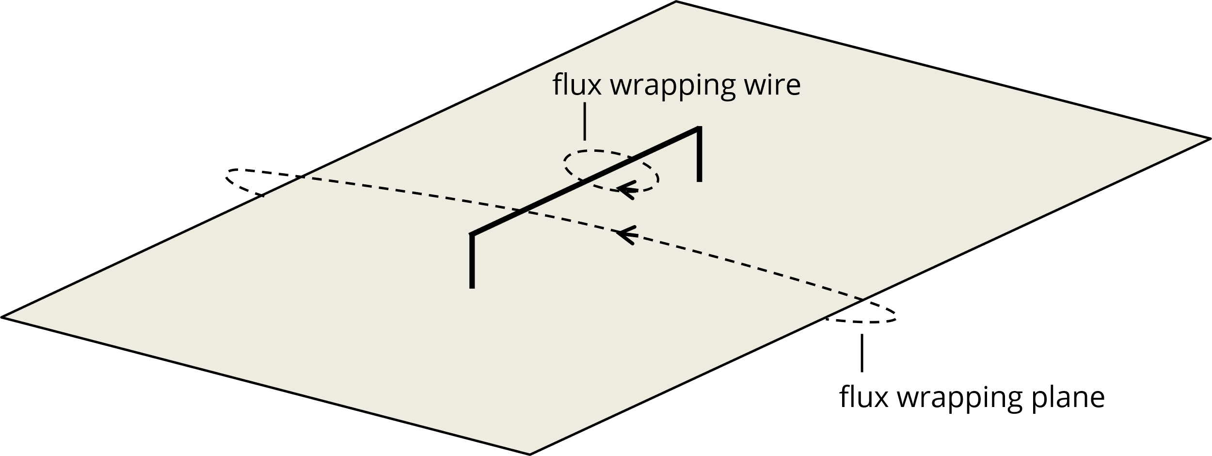
Consider the circuit loop shown in Figure 5. A wire half-loop extends above the surface of a finite-sized plane. Current flowing in the wire returns to its source through the plane. The height of the half-loop is small relative to the length of the half-loop and the width of the plane.

Figure 5. A wire half-loop above a plane.

The branch inductance of each piece of the loop is defined as the flux coupling the loop that encircles the current in that piece divided by the magnitude of the current. Summing the branch inductances of every piece in a loop yields the self-inductance of the loop.

Branch inductance is a convenient way of expressing the contribution that each part of a circuit makes to the total loop inductance. For the geometry in Figure 5, most of the flux in the loop is due to the current in the horizontal wire. The vertical wires contribute less flux due to their relatively short length. The plane contributes very little because the magnetic field wraps all the way around its width, significantly reducing the amplitude of the flux. Since the branch inductance of the horizontal wire accounts for nearly all of the total inductance, changes to that wire have a much more significant effect on the loop inductance than changes to the other parts of the circuit.

For a circuit board trace over a wide current return plane, the loop inductance is essentially equal to the branch inductance per unit length of the trace times the trace length. This branch inductance is commonly referred to as the trace inductance, but it is important to remember that it is not simply a property of the trace geometry. Branch inductances depend on the loop geometry. In order to assign an inductance to one branch, it is necessary to account for the entire current path.

It is not uncommon to see the term partial inductance used to describe a branch inductance. For example, one might refer to the partial inductance of a via, trace or plane in a signal path. In most cases, the intent is clear, and the choice of terms is not a problem. However, it’s important to recognize that this partial inductance and the partial inductance defined in the previous section are very different quantities. Calculations of the partial self-inductance as defined in the previous section do not yield a result equivalent to the branch inductance of a via, trace or plane.

Inductance of a Wire or Ground Strap

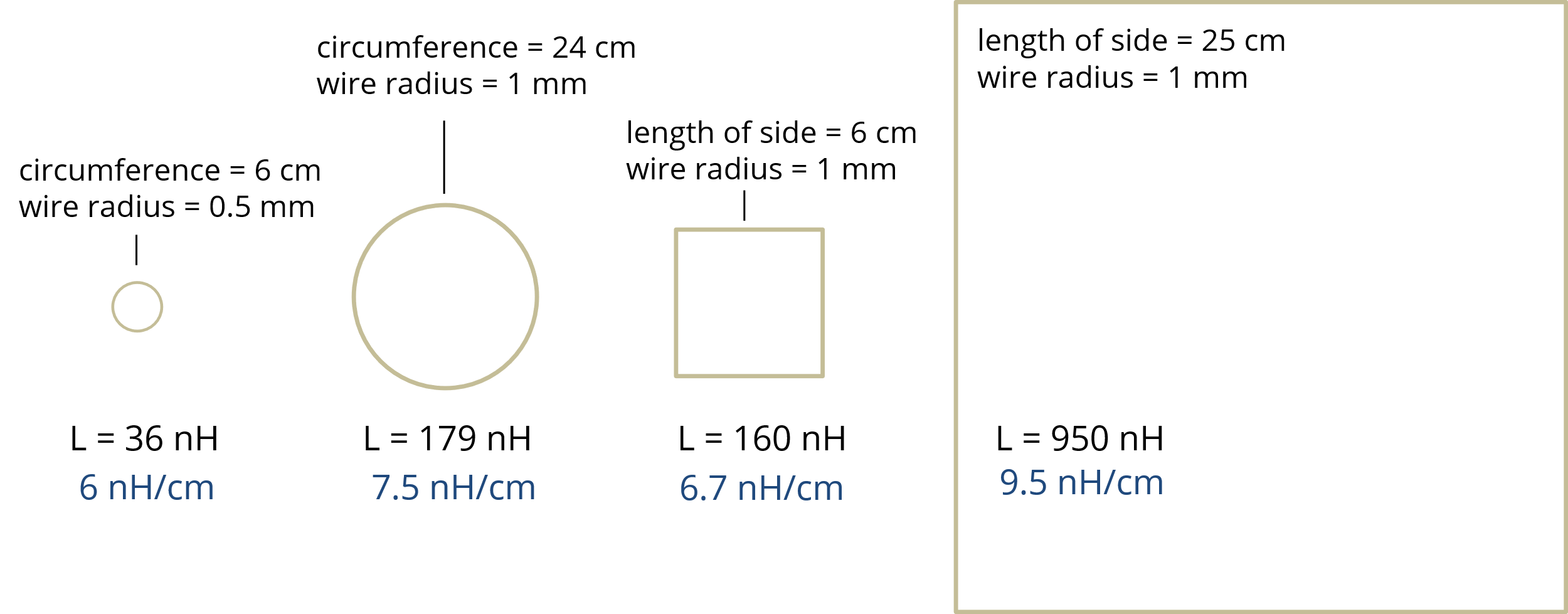
Figure 6. Wire loop geometries.

By now, it should be clear that inductance is a property of loops and that a wire, ground strap, or any conductor not part of a well-defined loop does not have a well-defined inductance. Nevertheless, estimating the branch inductance of components such as ground straps and vias is extremely important when modeling high-frequency circuits and systems. The inductance of these components cannot be ignored, just because it is not well-defined.

Fortunately, the branch inductance of these components can often be estimated even when the rest of the loop has not been precisely identified. To illustrate this, consider the four wire loops in Figure 6. These loops are shown approximately to scale relative to one another. The first loop is circular with a loop radius of only 3 mm. The wire radius is 0.5 mm. The second loop is also circular with a loop radius of 3 cm and a 1-mm wire radius. The third loop is square but has the same circumference as the second loop. The fourth loop is also square, but its sides are five times longer (and its loop area is 25 times larger) than those of the third loop. The calculated inductances for each loop are shown along with the inductance divided by the length of the wire (loop perimeter).

Note that even though the loop sizes and shapes are different, the inductance per unit length is on the order of 10 nH/cm. This is a useful approximation to keep in mind. As long as the return path is not too close, multiplying the length of a wire or strap by 10 nH/cm yields a reasonable order-of-magnitude estimate of its branch inductance.

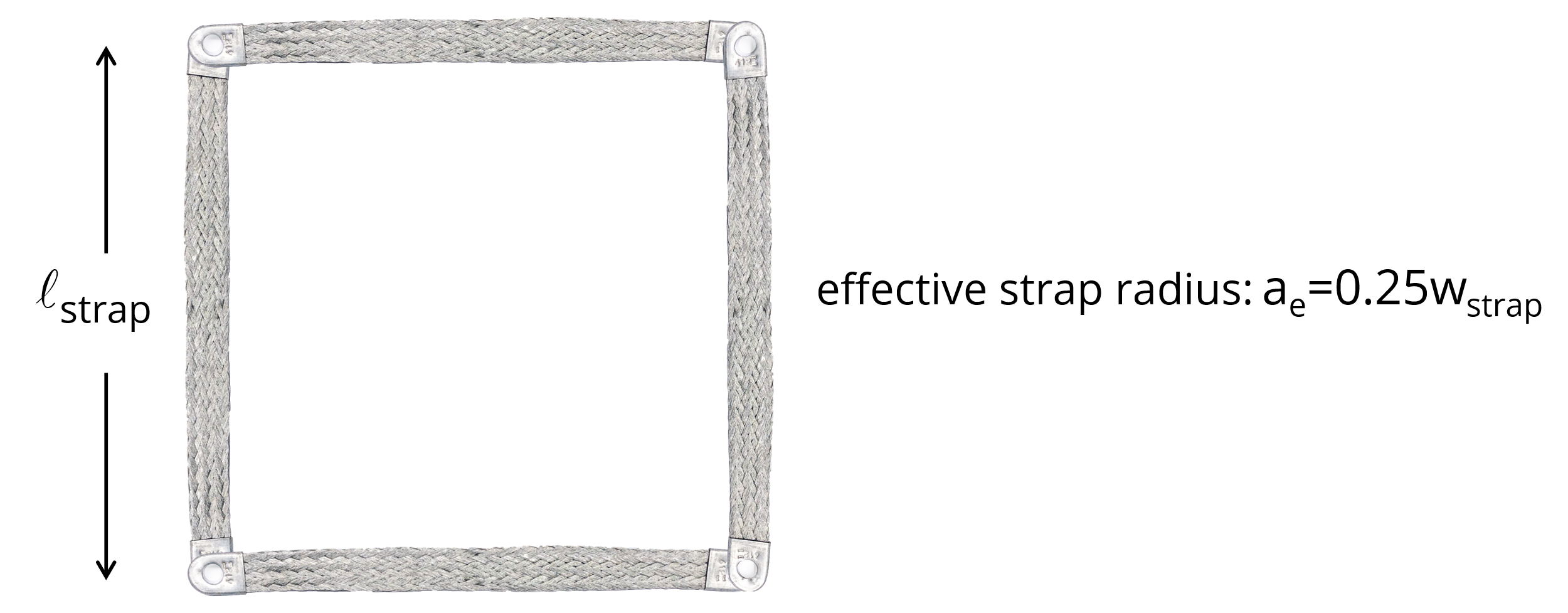
Figure 7. Square loop formed from ground straps.

We can make this approximation more accurate by accounting for the cross-sectional dimensions of the wire or strap. Consider the square loop formed by connecting four identical ground straps as shown in Figure 7. Equation (3) can be used to calculate the inductance of a square loop formed with round wire. These ground straps are not round wires, but we can use the same equation by recognizing that flat rectangular conductors with a width, w, have an effective radius,

(12)

ae = 0.25 w.

Applying (3) to calculate the inductance of the loop in Figure 7, we get

(13)

L= 2 μ 0 strap π ln 4 strap w strap 0.774 MathType@MTEF@5@5@+= feaahWart1ev3aaatCvAUfeBSjuyZL2yd9gzLbvyNv2CaerbpbxzUb YuH52CaeXatLxBI9gBaebbnrfifHhDYfgaruatPjwzYfgDP9MBGmvz YLMzaibaiKc9yrVq0xXdbba91rFfpec8Eeeu0xXdbba9frFj0=OqFf ea0dXdd9vqaq=JfrVkFHe9pgea0dXdar=Jb9hs0dXdbPYxe9vr0=vr 0=vqpWqaaeaabaGaaiaacaqabeaadaabamaaaOqaaiaadYeacqGH9a qpdaWcaaqaaiaaikdacqaH8oqBdaWgaaWcbaGaaGimaaqabaGccqqI tecBdaWgaaWcbaGaam4CaiaadshacaWGYbGaamyyaiaadchaaeqaaa GcbaGaeqiWdahaamaadmaabaGaciiBaiaac6gadaqadaqaamaalaaa baGaaGinaiabjoriSnaaBaaaleaacaWGZbGaamiDaiaadkhacaWGHb GaamiCaaqabaaakeaacaWG3bWaaSbaaSqaaiaadohacaWG0bGaamOC aiaadggacaWGWbaabeaaaaaakiaawIcacaGLPaaacqGHsislcaaIWa GaaiOlaiaaiEdacaaI3aGaaGinaaGaay5waiaaw2faaaaa@5BFA@ .

This result can then be divided by the circumference of the loop to get the inductance per unit length,

(14)

L 4 strap = μ 0 2π ln 4 strap w strap 0.774 = μ 0 2π ln 2 +ln 2× strap w strap 0.774 2× 10 7 ln 2× strap w strap henries/m 20 ln 2× strap w strap nH/cm. MathType@MTEF@5@5@+= feaahWart1ev3aaatCvAUfeBSjuyZL2yd9gzLbvyNv2CaerbpbxzUb YuH52CaeXatLxBI9gBaebbnrfifHhDYfgaruatPjwzYfgDP9MBGmvz YLMzaibaiKc9yrVq0xXdbba91rFfpec8Eeeu0xXdbba9frFj0=OqFf ea0dXdd9vqaq=JfrVkFHe9pgea0dXdar=Jb9hs0dXdbPYxe9vr0=vr 0=vqpWqaaeaabaGaaiaacaqabeaadaabamaaaOabaqqabaWaaSaaae aacaWGmbaabaGaaGinaiabjoriSnaaBaaaleaacaWGZbGaamiDaiaa dkhacaWGHbGaamiCaaqabaaaaOGaeyypa0ZaaSaaaeaacqaH8oqBda WgaaWcbaGaaGimaaqabaaakeaacaaIYaGaeqiWdahaamaadmaabaGa ciiBaiaac6gadaqadaqaaiaaisdadaWadaqaamaalaaabaGaeK4eHW 2aaSbaaSqaaiaadohacaWG0bGaamOCaiaadggacaWGWbaabeaaaOqa aiaadEhadaWgaaWcbaGaam4CaiaadshacaWGYbGaamyyaiaadchaae qaaaaaaOGaay5waiaaw2faaaGaayjkaiaawMcaaiabgkHiTiaaicda caGGUaGaaG4naiaaiEdacaaI0aaacaGLBbGaayzxaaGaaGjbVlaays W7aeaacaqG9aWaaSaaaeaacqaH8oqBdaWgaaWcbaGaaGimaaqabaaa keaacaaIYaGaeqiWdahaamaadmaabaGaaiiBaiaac6gadaqadaqaai aaikdaaiaawIcacaGLPaaacqGHRaWkciGGSbGaaiOBamaabmaabaWa aSaaaeaacaqGYaGaey41aqRaeK4eHW2aaSbaaSqaaiaadohacaWG0b GaamOCaiaadggacaWGWbaabeaaaOqaaiaadEhadaWgaaWcbaGaam4C aiaadshacaWGYbGaamyyaiaadchaaeqaaaaaaOGaayjkaiaawMcaai abgkHiTiaaicdacaGGUaGaaG4naiaaiEdacaaI0aGaaGjbVdGaay5w aiaaw2faaiaaysW7aeaacqGHijYUcaqGYaGaey41aqRaaeymaiaabc dadaahaaWcbeqaaiabgkHiTiaaiEdaaaGcdaWadaqaaiGacYgacaGG UbWaaeWaaeaadaWcaaqaaiaabkdacqGHxdaTcqqItecBdaWgaaWcba Gaam4CaiaadshacaWGYbGaamyyaiaadchaaeqaaaGcbaGaam4Damaa BaaaleaacaWGZbGaamiDaiaadkhacaWGHbGaamiCaaqabaaaaaGcca GLOaGaayzkaaGaaGjbVdGaay5waiaaw2faaiaaysW7caqGObGaaeyz aiaab6gacaqGYbGaaeyAaiaabwgacaqGZbGaae4laiaab2gaaeaacq GHijYUcaqGYaGaaGimamaadmaabaGaciiBaiaac6gadaqadaqaamaa laaabaGaaeOmaiabgEna0kabjoriSnaaBaaaleaacaWGZbGaamiDai aadkhacaWGHbGaamiCaaqabaaakeaacaWG3bWaaSbaaSqaaiaadoha caWG0bGaamOCaiaadggacaWGWbaabeaaaaaakiaawIcacaGLPaaaca aMe8oacaGLBbGaayzxaaGaaGjbVlaab6gacaqGibGaae4laiaaboga caqGTbGaaeOlaaaaaa@CFCA@

Multiplying the result in (14) by the length of the strap yields the branch inductance of one strap in this loop,

(15)

L20 strap ln 2× strap w strap nH. MathType@MTEF@5@5@+= feaahWart1ev3aaatCvAUfeBSjuyZL2yd9gzLbvyNv2CaerbpbxzUb YuH52CaeXatLxBI9gBaebbnrfifHhDYfgaruatPjwzYfgDP9MBGmvz YLMzaibaiKc9yrVq0xXdbba91rFfpec8Eeeu0xXdbba9frFj0=OqFf ea0dXdd9vqaq=JfrVkFHe9pgea0dXdar=Jb9hs0dXdbPYxe9vr0=vr 0=vqpWqaaeaabaGaaiaacaqabeaadaabamaaaOqaaiaadYeacqGHij YUcaqGYaGaaGimaiabjoriSnaaBaaaleaacaWGZbGaamiDaiaadkha caWGHbGaamiCaaqabaGcdaWadaqaaiGacYgacaGGUbWaaeWaaeaada WcaaqaaiaabkdacqGHxdaTcqqItecBdaWgaaWcbaGaam4Caiaadsha caWGYbGaamyyaiaadchaaeqaaaGcbaGaam4DamaaBaaaleaacaWGZb GaamiDaiaadkhacaWGHbGaamiCaaqabaaaaaGccaGLOaGaayzkaaGa aGjbVdGaay5waiaaw2faaiaaysW7caqGUbGaaeisaiaab6caaaa@5BE1@

We would have obtained a similar result if the loop had been any other relatively open shape. For this reason, it is convenient to use (15) to estimate the branch inductance of ground straps used in applications where the rest of the loop is undefined, but not tightly coupled to the strap.